Note

This page was generated from a Jupyter notebook. Not all interactive visualization will work on this web page. Consider downloading the notebooks for full Python-backed interactivity.

# holoviews initialization

5. Initialization

In order to run CNMF, we first need to generate an initial estimate of where our cells are likely to be and what their temporal activity is likely to look like. The whole initialization section is adapted from the MIN1PIPE package. See the paper for full details about the theory.

5.1. compute max projection

Here we calculate a max projection that will be used later. We also save this max projection in the output data folder, since it will be useful when carrying out cross-session registrations.

max_proj = save_minian(
    Y_fm_chk.max("frame").rename("max_proj"), **param_save_minian
).compute()

5.2. generating over-complete set of seeds

We first generate an over-complete set of seeds. Recall the parameters:

param_seeds_init

{'wnd_size': 1000,
 'method': 'rolling',
 'stp_size': 500,
 'max_wnd': 15,
 'diff_thres': 3}

The idea is that we select some subset of frames, compute a max projection of those frames, and find the local maxima of that max projection. We keep repeating this process and we collect all the local maxima until we obtain an overly-complete set of local maximas, which are the potential locations of cells, which we call seeds. The assumption here is that the center of cells are brighter than their surroundings on some, but not necessarily all, frames. There are several parameters controlling how we subset the frames: By default we use method="rolling", which use a rolling window across time to chunk and compute max projections. wnd_size controls the number of frames in each chunk. stp_size is the distance between the center of each chunk. For example, if wnd_size=100 and stp_size=50, the windows will be as follows: (0, 100), (50, 150), (100, 200)… Alternatively you can use method="random" to use random sampling of frames instead of rolling window. See the API reference of seeds_init for details. Additionally we have two parameters controlling how the local maxima are found. max_wnd controls the window size within which a single pixel will be choosen as local maxima. In order to capture cells with all sizes, we actually find local maximas with different window size and merge all of them, starting from 2 all the way up to max_wnd. Hence max_wnd should be the radius of the largest cell you want to detect. Finally in order to get rid of local maxima with very little fluctuation, we set a diff_thres which is the minimal fluorescent diffrence of a seed across frames. Since the linear scale of the raw data is preserved, we can set this threshold empirically.

%%time
seeds = seeds_init(Y_fm_chk, **param_seeds_init)

constructing chunks
computing max projections
calculating local maximum
CPU times: user 740 ms, sys: 104 ms, total: 844 ms
Wall time: 12.2 s

The seeds variable is a pandas.DataFrame, with each row representing a seed. The column “height” and “width” defines the location of the seed. The column “seeds” is the number of chunks where the particular seed/pixel is considered a local maxima.

seeds.head()

	height	width	seeds
0	0	325	1.0
1	0	381	1.0
2	0	387	1.0
3	1	263	2.0
4	2	352	1.0

We can visualize the seeds as points overlaid on top of the max_proj image. Each white dot is a seed and could potentially be the location of a cell.

hv.output(size=output_size)
visualize_seeds(max_proj, seeds)

5.3. peak-noise-ratio refine

Next, we refine seeds based upon their temporal activity. This requires that we separate our signal from noise based upon frequency. To find the best cut-off frequency, we are going to take a few example seeds and separate their activity with different cut-off frequencies. We will then view the results and select a frequency which we believe best separates signal from noise.

This is a complicated part in the pipeline, but it is important to understand since the idea is used later and it will allow you to do parameter exploration based on your need. The basic idea is to run some function on a small subset of the data using different parameters within a for loop, and then visualizing the results using holoviews.

We will go line by line:

1. First we create a list of frequencies we want to test – noise_freq_list. The “frequency” values here are a fraction of your sampling rate. Note that if you have temporally downsampled, the fraction here is relative to the downsampled rate.

2. Then we randomly select 6 rows from seeds and call them example_seeds.

3. Then we pull out the corresponding temporal activities of the 6 selected seeds and assign it to example_trace.

4. We then create an empty dictionary smooth_dict to store the resulting visualizations.

5. After initializing these variables, we use a for loop to iterate through noise_freq_list, with one of the values from the list as freq during each iteration.

6. Within the loop, we run smooth_sig twice on example_trace with the current freq we are testing out. The low-passed result is assigned to trace_smth_low, while the high-pass result is assigned to trace_smth_high.

7. Then we make sure to actually carry-out the computation by calling the compute method on the resulting DataArrays.

8. Next, we turn the two traces into visualizations: we construct interactive line plots (hv.Curves) from them and put them in a container called a hv.HoloMap.

9. Finally, we store the whole visualization in smooth_dict, with the keys being the freq and values corresponding to the result of this iteration.

So if you want to customize the parameter values to explore, in this case the cut-off frequency to test, you can edit noise_freq_list.

%%time
if interactive:
    noise_freq_list = [0.005, 0.01, 0.02, 0.06, 0.1, 0.2, 0.3, 0.45, 0.6, 0.8]
    example_seeds = seeds.sample(6, axis="rows")
    example_trace = Y_hw_chk.sel(
        height=example_seeds["height"].to_xarray(),
        width=example_seeds["width"].to_xarray(),
    ).rename(**{"index": "seed"})
    smooth_dict = dict()
    for freq in noise_freq_list:
        trace_smth_low = smooth_sig(example_trace, freq)
        trace_smth_high = smooth_sig(example_trace, freq, btype="high")
        trace_smth_low = trace_smth_low.compute()
        trace_smth_high = trace_smth_high.compute()
        hv_trace = hv.HoloMap(
            {
                "signal": (
                    hv.Dataset(trace_smth_low)
                    .to(hv.Curve, kdims=["frame"])
                    .opts(frame_width=300, aspect=2, ylabel="Signal (A.U.)")
                ),
                "noise": (
                    hv.Dataset(trace_smth_high)
                    .to(hv.Curve, kdims=["frame"])
                    .opts(frame_width=300, aspect=2, ylabel="Signal (A.U.)")
                ),
            },
            kdims="trace",
        ).collate()
        smooth_dict[freq] = hv_trace

CPU times: user 1.1 s, sys: 106 ms, total: 1.2 s
Wall time: 10.2 s

At the end of the process, we put together a smooth_dict. Here we convert that into an interactive plot, from which we can determine the frequency that best separates noise and signal.

hv.output(size=int(output_size * 0.7))
if interactive:
    hv_res = (
        hv.HoloMap(smooth_dict, kdims=["noise_freq"])
        .collate()
        .opts(aspect=2)
        .overlay("trace")
        .layout("seed")
        .cols(3)
    )
    display(hv_res)

noise_freq:

picking noise frequency

We can now use the interactive visualization to pick the best cut-off frequency. Here is an example of what you might see:

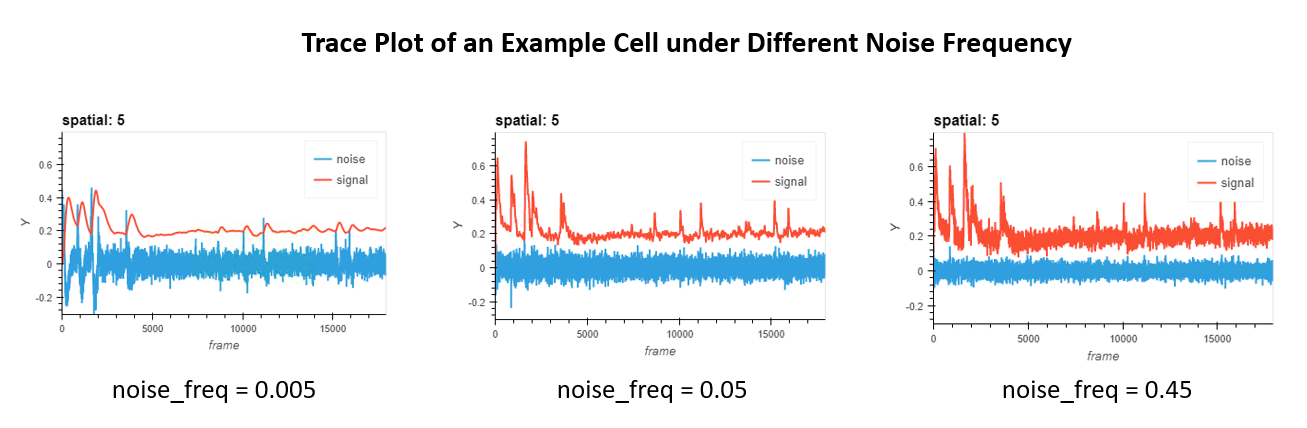
We are looking for the frequency that can best seperate real signal from noise. Hence, noise_freq=0.005 in the example is not ideal, since real calcium activities are overly smoothed as well. At the same time, noise_freq=0.45 is not ideal either, since a lot of high-frequency noise are visible in the signal. Hence, noise_freq=0.05 in the middle is a good choice in this example. Now, say you already found your parameters, it’s time now to pass them in! Either go back to initial parameters setting step and modify them there, or call the parameter here and change its value/s accordingly.

Having determined the frequency that best separates signal from noise, we move on to peak-noise-ratio refining. Recall the parameters:

param_pnr_refine

{'noise_freq': 0.06, 'thres': 1}

First we filter the temporal activities for each seed using the noise_freq we choose. signal is defined as the low-pass filtered temporal signal, while noise is high-pass filtered signal. Then we compute the peak-to-peak value (max minus min) for both the real signal and noise signal. The peak-noise-ratio is defined as the ratio between the peak-to-peak value of signal and that of noise. We then threshold the seeds based on this peak-noise-ratio, with the assumption that temporal activities from real cells should have higher fluctuation in the low-frequency range and lower fluctuation in the high-frequency range. thres is the threshold for peak-noise-ratios. Pragmatically thres=1 works fine and makes sense. You can also use thres="auto", where a gaussian mixture model with 2 components will be run on the peak-noise-ratios and seeds will be selected if they belong to the “higher” gaussian.

The following cell would carry out pnr refinement step. Be sure to change the noise_freq based on visualization results before running the following cell.

%%time
seeds, pnr, gmm = pnr_refine(Y_hw_chk, seeds, **param_pnr_refine)

selecting seeds
computing peak-noise ratio
CPU times: user 2.73 s, sys: 187 ms, total: 2.92 s
Wall time: 36 s

The resulting seeds dataframe will have an additional column “mask_pnr” showing you whether a seed passed the peak-noise-ratio threshold.

seeds.head()

	height	width	seeds	mask_pnr
0	0	325	1.0	False
1	0	381	1.0	False
2	0	387	1.0	False
3	1	263	2.0	False
4	2	352	1.0	False

If you chose thres="auto" you can use the following cell to visualize the gaussian mixture model fit.

if gmm:
    display(visualize_gmm_fit(pnr, gmm, 100))
else:
    print("nothing to show")

nothing to show

We can visualize seeds on top of the max projection again. This time we can also pass in “mask_pnr” so that the visualization can show us which seeds are filtered out in pnr_refine. White dots are accepted seeds and red dots are taken out.

If you see seeds being filtered out that you believe should be cells, either skip this step or try lower the threshold a bit.

hv.output(size=output_size)
visualize_seeds(max_proj, seeds, "mask_pnr")

5.4. ks refine

ks_refine refines the seeds using Kolmogorov-Smirnov test. Recall the parameters:

param_ks_refine

{'sig': 0.05}

The idea is simple: if a seed corresponds to a cell, its fluorescence intensity across frames should be distributed following a bimodal distribution, with a large peak representing noise/little activity, and another peak representing when the seed/cell is active. Thus, we can carry out KS test on the distribution of fluorescence intensity of each seed, and keep only the seeds where the null hypothesis (that the fluorescence is just a normal distribution) is rejected. sig is the p value at which the null hypothesis is rejected.

%%time
seeds = ks_refine(Y_hw_chk, seeds, **param_ks_refine)

selecting seeds
performing KS test
CPU times: user 2.45 s, sys: 223 ms, total: 2.68 s
Wall time: 36.3 s

We can visualize seeds on top of the max projection. White dots are accepted seeds and red dots are taken out.

The ks refine step tend to have minimal impact. It’s quite normal to see no seeds being filtered out and you can proceed in such cases.

hv.output(size=output_size)
visualize_seeds(max_proj, seeds, "mask_ks")

5.5. merge seeds

At this point, much of our refined seeds likely reflect the position of an actual cell. However, we are likely to still have multiple seeds per cell, which we want to avoid. Here we discard redundant seeds through a process of merging. Recall the parameters:

param_seeds_merge

{'thres_dist': 10, 'thres_corr': 0.8, 'noise_freq': 0.06}

The function seeds_merge attempts to merge seeds together which potentially come from the same cell, based upon their spatial distance and temporal correlation. Specifically, thres_dist is the threshold for euclidean distance between pairs of seeds, in pixels, and thres_corr is the threshold for pearson correlation between pairs of seeds. In addition, it’s very beneficial to smooth the signals before computing the correlation, and noise_freq determines how smoothing should be done. Any pair of seeds that are within thres_dist and has a correlation higher than thres_corr will be merged together, such that only the seed with maximum intensity in the max projection of the video will be kept.

Note that we apply the masking from previous refining steps here and use only those seeds as input to seeds_merge.

Since the merge is carried out transitively, in practice it is beneficial to keep thres_dist small to avoid over-merging, especially when the density of cells is high. The goal of this step is to reduce the number of duplicated seeds as much as possible, but not over-merge the seeds, since merging is irreversible. Hence it is OK to have multiple seeds per cell at this stage.

%%time
seeds_final = seeds[seeds["mask_ks"] & seeds["mask_pnr"]].reset_index(drop=True)
seeds_final = seeds_merge(Y_hw_chk, max_proj, seeds_final, **param_seeds_merge)

computing distance
computing correlations
pixel recompute ratio: 0.849493487698987
computing correlations
merging seeds
CPU times: user 1.64 s, sys: 47.6 ms, total: 1.69 s
Wall time: 6.4 s

We visualize the result on top of the max projection. The red dots here indicate seeds that has been merged to nearby seeds (those shown in white).

hv.output(size=output_size)
visualize_seeds(max_proj, seeds_final, "mask_mrg")

5.6. initialize spatial matrix

Up till now, the seeds we have are only one-pixel dots. In order to kick start CNMF we need something more like the spatial footprint (A) and temporal activities (C) of real cells. Thus we need to initilalize A and C from the seeds we have. Recall the parameters:

param_initialize

{'thres_corr': 0.8, 'wnd': 10, 'noise_freq': 0.06}

To obtain the initial spatial matrix A, for each seed, we calculate Pearson correlation between the seed and surrounding pixels. Calculating correlation with all other pixels for every seed is time-consuming and unnecessary. Hence we use wnd to control the window size for calculating the correlation, and thus is the maximum possible size of any spatial footprint in the initial spatial matrix. At the same time we do not want pixels with low correlation value to influence our estimation of temporal signals, thus a thres_corr is also implemented where only pixels with correlation above this threshold are kept.

%%time
A_init = initA(Y_hw_chk, seeds_final[seeds_final["mask_mrg"]], **param_initialize)
A_init = save_minian(A_init.rename("A_init"), intpath, overwrite=True)

optimizing computation graph
pixel recompute ratio: 1.0543114067504311
computing correlations
building spatial matrix
CPU times: user 20.3 s, sys: 752 ms, total: 21 s
Wall time: 1min 2s

5.7. initialize temporal matrix

After generating A, for each seed, we calculate a weighted average of pixels around the seed, where the weight are the initial spatial footprints in A we just generated. We use this weighted average as the initial estimation of temporal activities for each units in C.

%%time
C_init = initC(Y_fm_chk, A_init)
C_init = save_minian(
    C_init.rename("C_init"), intpath, overwrite=True, chunks={"unit_id": 1, "frame": -1}
)

CPU times: user 2.88 s, sys: 321 ms, total: 3.2 s
Wall time: 1min 19s

5.8. merge units

We want to do another pass of merging before proceeding, and this time we want to merge based on initialized A and C. Recall the parameters:

param_init_merge

{'thres_corr': 0.8}

The unit_merge consider all cells whose spatial footprints have at least one pixel in common to be potential target of merging. Hence, the only parameter you need to specify is a threshold for the correlation of the temporal activities of cells to be merged.

%%time
A, C = unit_merge(A_init, C_init, **param_init_merge)
A = save_minian(A.rename("A"), intpath, overwrite=True)
C = save_minian(C.rename("C"), intpath, overwrite=True)
C_chk = save_minian(
    C.rename("C_chk"),
    intpath,
    overwrite=True,
    chunks={"unit_id": -1, "frame": chk["frame"]},
)

computing spatial overlap
computing temporal correlation
pixel recompute ratio: 0.34448160535117056
computing correlations
labeling units to be merged
merging units
CPU times: user 5.32 s, sys: 112 ms, total: 5.43 s
Wall time: 13.3 s

5.9. initialize background terms

Finally, we need two more terms: b and f, representing the spatial footprint and temporal dynamics of the background, respectively. We first compute an estimation of cellular activities by taking the outer product of A and C, resulting in an video array with dimesion height, width and frame. We then subtract this array from Y_fm_chk, resulting in a “residule” movie. Then b is estimated as the mean projection of the “residule” movie, while f is estimated as the fluorescence fluctuation of b that best fit the “residule” movie (least-square solution).

%%time
b, f = update_background(Y_fm_chk, A, C_chk)
f = save_minian(f.rename("f"), intpath, overwrite=True)
b = save_minian(b.rename("b"), intpath, overwrite=True)

CPU times: user 2.12 s, sys: 160 ms, total: 2.28 s
Wall time: 32.6 s

5.10. visualization of initialization

Finally we visualize the result of our initialization by plotting a projection of the spatial matrix A, a raster of the temporal matrix C, as well as background terms b and f.

hv.output(size=int(output_size * 0.55))
im_opts = dict(
    frame_width=500,
    aspect=A.sizes["width"] / A.sizes["height"],
    cmap="Viridis",
    colorbar=True,
)
cr_opts = dict(frame_width=750, aspect=1.5 * A.sizes["width"] / A.sizes["height"])
(
    regrid(
        hv.Image(
            A.max("unit_id").rename("A").compute().astype(np.float32),
            kdims=["width", "height"],
        ).opts(**im_opts)
    ).relabel("Initial Spatial Footprints")
    + regrid(
        hv.Image(
            C.rename("C").compute().astype(np.float32), kdims=["frame", "unit_id"]
        ).opts(cmap="viridis", colorbar=True, **cr_opts)
    ).relabel("Initial Temporal Components")
    + regrid(
        hv.Image(
            b.rename("b").compute().astype(np.float32), kdims=["width", "height"]
        ).opts(**im_opts)
    ).relabel("Initial Background Sptial")
    + datashade(hv.Curve(f.rename("f").compute(), kdims=["frame"]), min_alpha=200)
    .opts(**cr_opts)
    .relabel("Initial Background Temporal")
).cols(2)

4. Motion Correction 6. CNMF